XLOOKUP vs VLOOKUP in Google Sheets: the 2-minute version

Takeaway

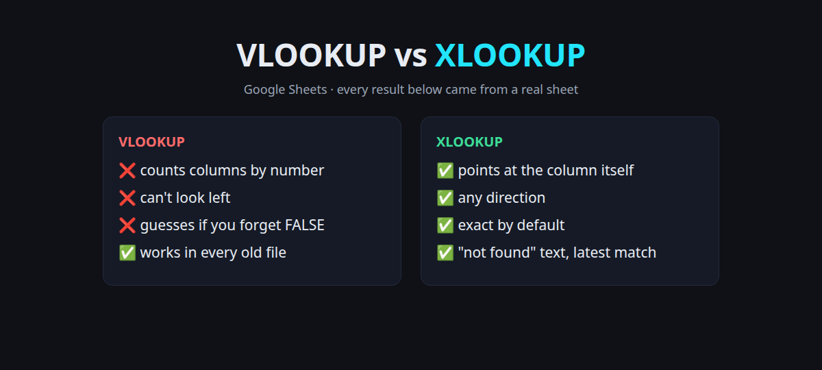
Use XLOOKUP for new sheets. VLOOKUP isn’t broken, but it counts columns by number and guesses when you forget FALSE. Both mistakes give you a wrong answer instead of an error.

I ran every formula below in a scratch Google Sheet on 2026-10-14. The results are what Sheets actually returned.

The test sheet

A tiny product list on a tab called Products:

	A: SKU	B: Product	C: Price	D: Stock
2	P-100	Notebook	4.50	12
3	P-101	Pen (blue)	1.20	40
4	P-102	Stapler	9.90	0
5	P-103	Marker set	7.25	5
6	P-104	Desk lamp	27.50	3

Side by side

Job	VLOOKUP	XLOOKUP	What I got
Price of P-102	`=VLOOKUP("P-102",A2:D6,3,FALSE)`	`=XLOOKUP("P-102",A2:A6,C2:C6)`	9.9 / 9.9
SKU of “Stapler” (look left)	`=VLOOKUP("Stapler",A2:D6,1,FALSE)`	`=XLOOKUP("Stapler",B2:B6,A2:A6)`	#N/A / P-102
Missing SKU	`=VLOOKUP("P-999",A2:D6,3,FALSE)`	`=XLOOKUP("P-999",A2:A6,C2:C6,"not found")`	#N/A / not found
Whole row for P-103	three formulas	`=XLOOKUP("P-103",A2:A6,B2:D6)`	Marker set, 7.25, 5

VLOOKUP only searches the first column of its range, so it can’t find “Stapler” and walk left to the SKU. XLOOKUP has a separate search range and result range, so direction doesn’t matter.

Trap 1: one inserted column

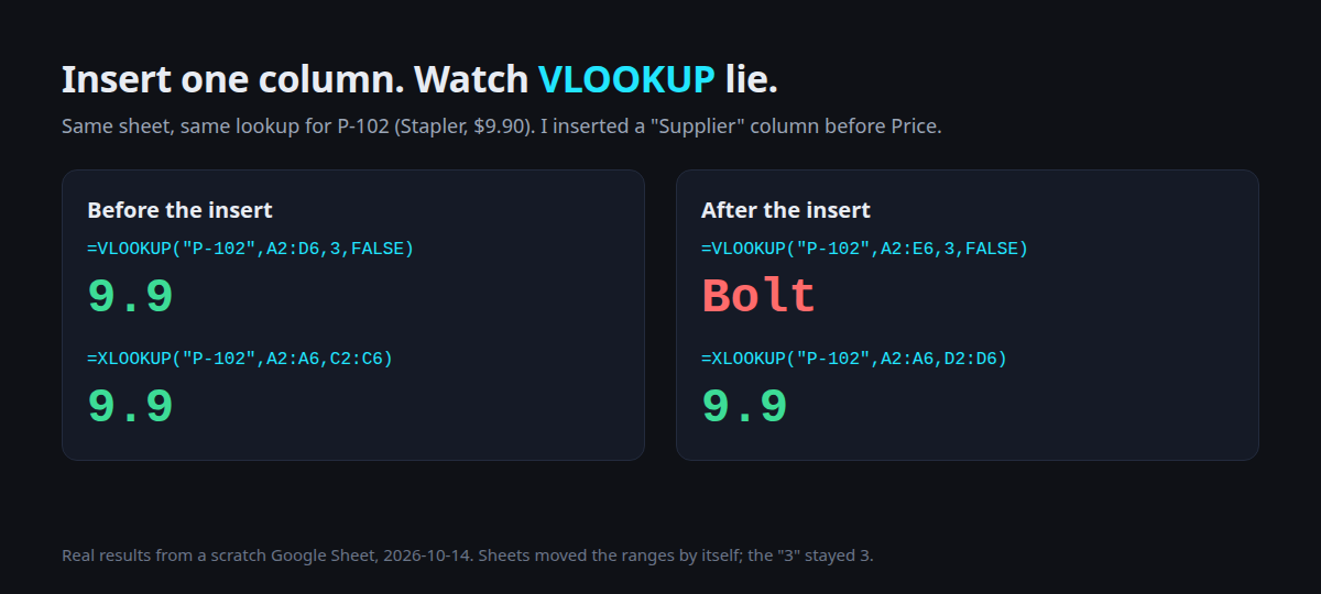
Before and after inserting a column: VLOOKUP returns Bolt, XLOOKUP still returns 9.9

I inserted a Supplier column between Product and Price. Sheets updated both ranges by itself, but VLOOKUP’s 3 stayed 3.

Column 3 is now Supplier, so the “price” became Bolt. No error, no warning, just a supplier name where a number should be.

XLOOKUP pointed at the Price column itself (C2:C6 became D2:D6) and still returned 9.9.

Trap 2: forgetting FALSE

=VLOOKUP("P-105", A2:D6, 3)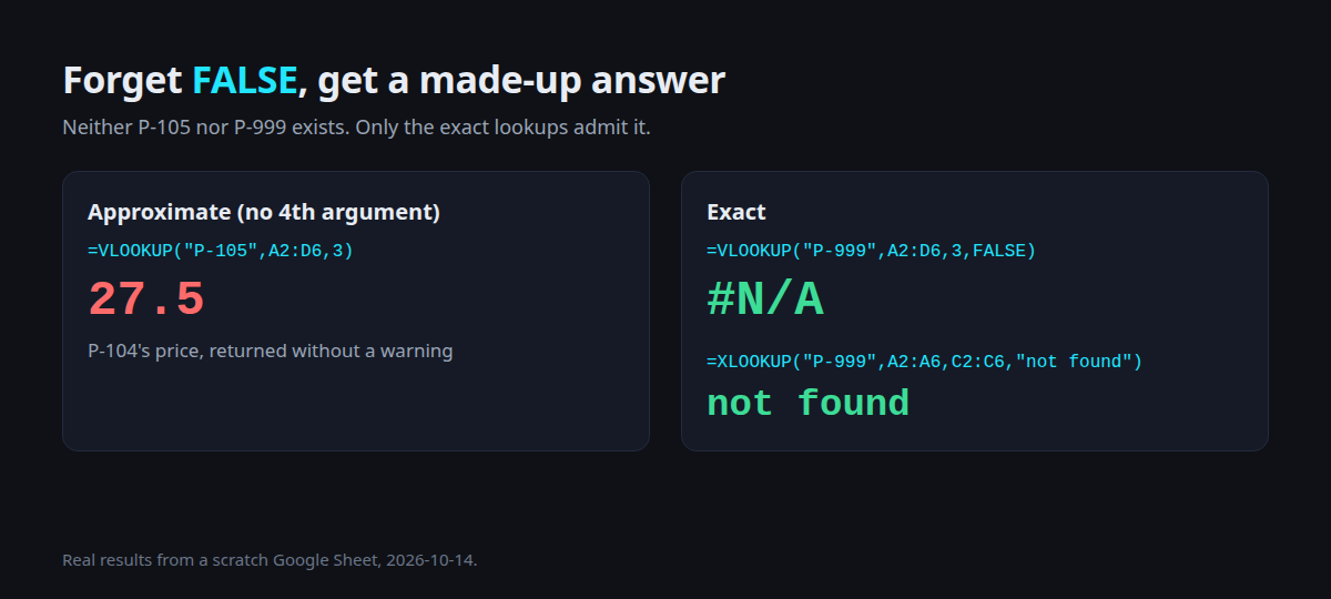

VLOOKUP without FALSE returns 27.5 for a missing SKU; exact lookups return #N/A or not found

P-105 doesn’t exist. Without the fourth argument VLOOKUP does an approximate match, so it returned 27.5, the price of P-104. A made-up product, a real-looking price.

XLOOKUP is exact by default. You only get approximate matching when you ask for it.

When you do want “closest”: discount tiers

Approximate matching is useful for tiers. A Tiers tab:

Min order	Discount
0	0%
50	5%
100	10%
200	15%

=XLOOKUP(130, Tiers!A2:A5, Tiers!B2:B5, , -1)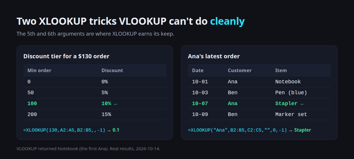

XLOOKUP picking the 10% tier for a 130 order and Ana's latest order, Stapler

The -1 means “exact, or the next smaller value”. An order of 130 got 0.1 (10%). =VLOOKUP(130,Tiers!A2:B5,2,TRUE) also gave 0.1, but only because the tiers are sorted ascending. XLOOKUP’s -1 doesn’t require sorting.

Bonus: the latest match, not the first

An order log with Ana on Oct 1 (Notebook) and again on Oct 7 (Stapler):

=XLOOKUP("Ana", Log!B2:B5, Log!C2:C5, "", 0, -1)

The last -1 searches bottom-up, so it returned Stapler, her latest order. VLOOKUP("Ana",…,FALSE) returned Notebook, the first one.

One that gets both of them

=XLOOKUP("Notebook ", B2:B6, C2:C6, "not found")   → not found
=XLOOKUP(TRIM("Notebook "), B2:B6, C2:C6, "not found")   → 4.5

A trailing space (very common after copy-paste from email) breaks exact matching in both functions. TRIM the key, or clean the column once.

Cheat sheet

You want	Write
Exact lookup	`=XLOOKUP(key, search_col, result_col)`
Friendly miss	add `, "not found"` as 4th argument
Several columns	make the result range wider: `B2:D6`
Tiers / brackets	`, , -1` (next smaller)
Latest entry	`, "", 0, -1` (search from bottom)
Old file with VLOOKUP	always end with `, FALSE`

If a sheet is shared with Excel users on old versions, VLOOKUP with FALSE is still fine. Just don’t hard-code the column number in a sheet people add columns to.

Got a sheet where lookups keep breaking every time someone adds a column? Send me what it does, and I’ll tell you whether a formula fix is enough or it needs a small script.